import icechunk
import obstore
import fnmatch

from virtualizarr import open_virtual_dataset, open_virtual_mfdataset
from virtualizarr.parsers import HDFParser
from virtualizarr.registry import ObjectStoreRegistry
import xarray as xrGenerate Virtual Zarr from CMIP6 NetCDF files
Tutorial for data providers who want to create a virtual icechunk store for NetCDF files.
Run this notebook
You can launch this notebook in VEDA JupyterHub by clicking the link below.
Launch in VEDA JupyterHub (requires access)
Learn more
Inside the Hub
This notebook was written on a VEDA JupyterHub instance using the default modified Pangeo image which contains all necessary libraries.
See VEDA Analytics JupyterHub Access for information about how to gain access.
Outside the Hub
You are welcome to run this anywhere you like (Note: alternatively you can run this on MAAP, locally, …), just make sure that you have a compatible environment and the data is accessible, or get in contact with the VEDA team to enable access.
Approach
This notebook demonstrates how to create a virtual Icechunk store reference for the AWS Open Data Registry of NASA Earth Exchange Global Daily Downscaled Projections (NEX-GDDP-CMIP6) NetCDF files on S3. Because the NetCDF files are publicly avaialble, this notebook should be runnable in any environment with the imported libraries, up until the last step where the Icechunk store is stored in the veda-data-store-staging S3 bucket, as that is a protected bucket.
To see how to publish a virtual Icechunk store to a STAC collection, see the Publishing CMIP6 Virtual Zarr to STAC notebook.
Step 1: Setup
Import necessary libraries and define some variables for which CMIP6 variable and model we will create references for.
Zarr can emit a lot of warnings about Numcodecs not being including in the Zarr version 3 specification yet – let’s suppress those.
import warnings

warnings.filterwarnings(
    "ignore",
    message="Numcodecs codecs are not in the Zarr version 3 specification*",
    category=UserWarning,
)
Specify the CMIP model and variable to use. Here we are using near-surface air temperature from the GISS-E2-1-G GCM.
Note: We are only using the historical data in this example.
More years of data are available from multiple Shared Socio-Economic Pathways (SSPs) in the s3://nex-gddp-cmip6 bucket.
model = "GISS-E2-1-G"
variable = "tas"

s3_bucket = "nex-gddp-cmip6"
s3_region = "us-west-2"
s3_anonymous = True  # set to false for a private bucket
s3_prefix = "NEX-GDDP-CMIP6/GISS-E2-1-G/historical/"
s3_path = f"s3://{s3_bucket}/{s3_prefix}"
file_pattern = f"{s3_prefix}r1i1p1*/{variable}/*"
Step 2: Initiate file systems for reading
We can use Obstore’s obstore.store.from_url convenience method to create an ObjectStore that can fetch data from the specified URLs.
store = obstore.store.from_url(f"s3://{s3_bucket}/", region="us-west-2", skip_signature=True)Step 3: Discover files from S3
List all available files for the model and then filter them to those that match the specified variable:
pages_of_files = obstore.list(store, prefix=s3_prefix)

all_files = []
async for files in pages_of_files:
    all_files += [f["path"] for f in files if fnmatch.fnmatch(f["path"], file_pattern)]

print(f"{len(all_files)} discovered matching s3://{s3_bucket}/{file_pattern}")
130 discovered matching s3://nex-gddp-cmip6/NEX-GDDP-CMIP6/GISS-E2-1-G/historical/r1i1p1*/tas/*Step 4: Open a single file as a virtual dataset
Now, let’s create a virtual dataset by passing the URL, a parser instance, and an ObjectStoreRegistry instance to virtualizarr.open_virtual_dataset.
We’ll try it with a single file first to make sure it works and get a sense of how long it takes to scan the NetCDF.
%%time
vds = open_virtual_dataset(
    url=f"s3://{s3_bucket}/{all_files[0]}",
    parser=HDFParser(),
    registry=ObjectStoreRegistry({f"s3://{s3_bucket}/": store}),
)
print(vds)
<xarray.Dataset> Size: 1GB
Dimensions: (time: 365, lat: 600, lon: 1440)
Coordinates:
* time (time) object 3kB 1950-01-01 12:00:00 ... 1950-12-31 12:00:00
* lat (lat) float64 5kB -59.88 -59.62 -59.38 -59.12 ... 89.38 89.62 89.88
* lon (lon) float64 12kB 0.125 0.375 0.625 0.875 ... 359.4 359.6 359.9
Data variables:
tas (time, lat, lon) float32 1GB ManifestArray<shape=(365, 600, 1440...
Attributes: (12/23)
downscalingModel: BCSD
activity: NEX-GDDP-CMIP6
contact: Dr. Rama Nemani: rama.nemani@nasa.gov, Dr. Bridget...
Conventions: CF-1.7
creation_date: 2021-10-04T18:41:40.796912+00:00
frequency: day
... ...
history: 2021-10-04T18:41:40.796912+00:00: install global a...
disclaimer: This data is considered provisional and subject to...
external_variables: areacella
cmip6_source_id: GISS-E2-1-G
cmip6_institution_id: NASA-GISS
cmip6_license: CC-BY-SA 4.0
CPU times: user 4.29 s, sys: 339 ms, total: 4.62 s
Wall time: 6.2 sStep 5: Open all the files as a virtual multifile dataset
Just like we can open one file as a virtual dataset using virtualizarr.open_virtual_dataset, we can open multiple data sources into a single virtual dataset using virtualizarr.open_virtual_mfdataset, similar to how xarray.open_mfdataset opens multiple data files as a single dataset.
Note this takes some time because VirtualiZarr needs to scan each file to extract its metadata. We can expect it to take at least 130 * whatever the last cell took.
%%time
vds = open_virtual_mfdataset(
    [f"s3://{s3_bucket}/{path}" for path in all_files],
    parser=HDFParser(),
    registry=ObjectStoreRegistry({f"s3://{s3_bucket}/": store}),
)
print(vds)
<xarray.Dataset> Size: 82GB
Dimensions: (time: 23725, lat: 600, lon: 1440)
Coordinates:
* time (time) object 190kB 1950-01-01 12:00:00 ... 2014-12-31 12:00:00
* lat (lat) float64 5kB -59.88 -59.62 -59.38 -59.12 ... 89.38 89.62 89.88
* lon (lon) float64 12kB 0.125 0.375 0.625 0.875 ... 359.4 359.6 359.9
Data variables:
tas (time, lat, lon) float32 82GB ManifestArray<shape=(23725, 600, 1...
Attributes: (12/22)
downscalingModel: BCSD
activity: NEX-GDDP-CMIP6
Conventions: CF-1.7
frequency: day
institution: NASA Earth Exchange, NASA Ames Research Center, Mo...
variant_label: r1i1p1f2
... ...
cmip6_institution_id: NASA-GISS
cmip6_license: CC-BY-SA 4.0
contact: Dr. Bridget Thrasher: bridget@climateanalyticsgrou...
creation_date: Sat Nov 16 21:42:29 PST 2024
disclaimer: These data are considered provisional and subject ...
tracking_id: ba64ebba-3c17-4348-b463-7e6ae7d11769
CPU times: user 16.8 s, sys: 18.3 s, total: 35.1 s
Wall time: 5min 30sThe size represents the size of the original dataset - you can see the size of the virtual dataset using the vz accessor:
print(f"Original dataset size: {vds.nbytes / 1000**3:.2f} GB")
print(f"Virtual dataset size: {vds.vz.nbytes / 1000:.2f} kB")
Original dataset size: 81.99 GB
Virtual dataset size: 965.32 kBThe magic of virtual Zarr is that you can persist the virtual dataset to disk in a chunk references format such as Icechunk or kerchunk, meaning that the work of constructing the single coherent dataset only needs to happen once. For subsequent data access, you can use xarray.open_zarr to open that virtual Zarr store, which on object storage is far faster than using xarray.open_mfdataset to open the the original non-cloud-optimized files.
Step 6: Write to Icechunk
Let’s persist the virtual dataset using Icechunk. Here there are two different options for storing the dataset. If you don’t have sufficient credentials you can store it in memory. Otherwise you can store the virtual dataset in the veda-data-store-staging bucket on s3.
icechunk_store = icechunk.s3_storage(
    bucket="veda-data-store-staging",
    region="us-west-2",
    prefix=f"cmip6-{model}-{variable}-historical-icechunk",
    from_env=True,
)
icechunk_store = icechunk.in_memory_storage()Did you pick where to write to?
Good! Let’s do it!
config = icechunk.RepositoryConfig.default()

config.set_virtual_chunk_container(
    icechunk.VirtualChunkContainer(
        url_prefix=s3_path,
        store=icechunk.s3_store(region=s3_region, anonymous=s3_anonymous),
    ),
)

if s3_anonymous:
    virtual_credentials = icechunk.containers_credentials(
        {s3_path: icechunk.s3_anonymous_credentials()}
    )

repo = icechunk.Repository.create(
    icechunk_store,
    config,
    authorize_virtual_chunk_access=virtual_credentials,
)

session = repo.writable_session("main")
vds.vz.to_icechunk(session.store)
session.commit("Create virtual store")'SHSZN93MQCNF93SE7M30'To make sure it worked, let’s take a look at the bucket:
!aws s3 ls s3://veda-data-store-staging/cmip6-GISS-E2-1-G-tas-historical-icechunk/ PRE manifests/
PRE refs/
PRE snapshots/
PRE transactions/
2025-09-18 16:23:48 447 config.yamlWhat about kerchunk?
NOTE: We tend to prefer Icechunk because it is scalable, ensures ACID transactions and has built-in version control. But you can write virtual datasets to kerchunk. Here is how you can write a local kerchunk-json file:
vds.vz.to_kerchunk(
    filepath=f"combined_CMIP6_daily_{model}_{variable}_kerchunk.json",
    format="json",
)
Final Step: Check your work
It is always a good idea to check your work when creating a new virtual dataset by comparing the virtual version to the native version. In this case let’s check the version on s3 so we can compare the times it takes to lazily open the virtual dataset compared to the native version.
%%time
storage = icechunk.s3_storage(
    bucket="veda-data-store-staging",
    region="us-west-2",
    prefix=f"cmip6-{model}-{variable}-historical-icechunk",
    from_env=True,
)

config = icechunk.RepositoryConfig.default()
config.set_virtual_chunk_container(
    icechunk.VirtualChunkContainer(
        s3_path,
        icechunk.s3_store(region=s3_region)
    )
)

if s3_anonymous:
    virtual_credentials = icechunk.containers_credentials(
        {
            s3_path: icechunk.s3_anonymous_credentials()
        }
    )

repo = icechunk.Repository.open(
    storage=storage,
    config=config,
    authorize_virtual_chunk_access=virtual_credentials,
)
session = repo.readonly_session(branch="main")

observed = xr.open_zarr(session.store)
observed
CPU times: user 157 ms, sys: 0 ns, total: 157 ms
Wall time: 391 ms<xarray.Dataset> Size: 82GB
Dimensions: (time: 23725, lat: 600, lon: 1440)
Coordinates:
* lat (lat) float64 5kB -59.88 -59.62 -59.38 -59.12 ... 89.38 89.62 89.88
* lon (lon) float64 12kB 0.125 0.375 0.625 0.875 ... 359.4 359.6 359.9
* time (time) object 190kB 1950-01-01 12:00:00 ... 2014-12-31 12:00:00
Data variables:
tas (time, lat, lon) float32 82GB dask.array<chunksize=(1, 600, 1440), meta=np.ndarray>
Attributes: (12/22)
downscalingModel: BCSD
activity: NEX-GDDP-CMIP6
Conventions: CF-1.7
frequency: day
institution: NASA Earth Exchange, NASA Ames Research Center, Mo...
variant_label: r1i1p1f2
... ...
cmip6_institution_id: NASA-GISS
cmip6_license: CC-BY-SA 4.0
contact: Dr. Bridget Thrasher: bridget@climateanalyticsgrou...
creation_date: Sat Nov 16 21:42:29 PST 2024
disclaimer: These data are considered provisional and subject ...
tracking_id: ba64ebba-3c17-4348-b463-7e6ae7d11769Make sure you can access the underlying chunk data. Let’s time this as well so we can compare it to the native version
%%time
data_slice = observed.tas.sel(time="2010", lat=slice(39, 41), lon=slice(284, 286))
data_slice.mean(dim="time").compute().plot()
CPU times: user 7.15 s, sys: 1.45 s, total: 8.6 s
Wall time: 7.45 s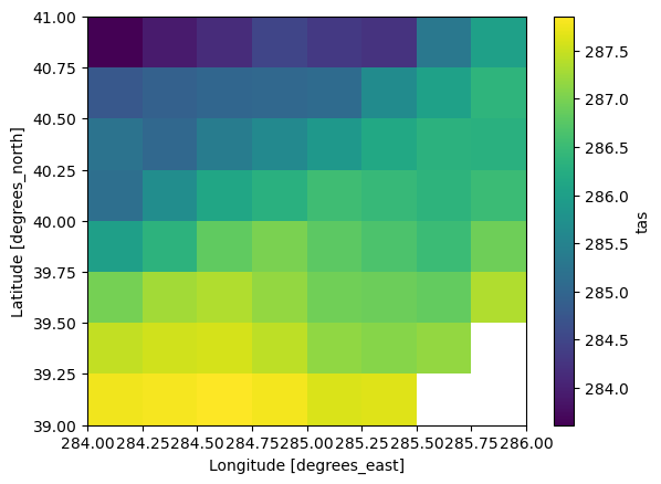
Compare that with the traditional method of opening the NetCDF files directly. We’ll tweak the fsspec configuration to fetch larger blocks at a time.
import fsspec

fs = fsspec.filesystem("s3", anon=True)

fsspec_kwargs = {
    "cache_type": "blockcache",  # block cache stores blocks of fixed size and uses eviction using a LRU strategy.
    "block_size": 8 * 1024 * 1024,  # size in bytes per block, depends on the file size but recommendation is in the MBs
}
Now we can lazily open all the NetCDF files.
%%time
expected = xr.open_mfdataset(
    [fs.open(f"s3://{s3_bucket}/{path}" , **fsspec_kwargs) for path in all_files],
    engine="h5netcdf"
)
expected
CPU times: user 10.6 s, sys: 2.5 s, total: 13.1 s
Wall time: 57.3 s<xarray.Dataset> Size: 82GB
Dimensions: (time: 23725, lat: 600, lon: 1440)
Coordinates:
* time (time) object 190kB 1950-01-01 12:00:00 ... 2014-12-31 12:00:00
* lat (lat) float64 5kB -59.88 -59.62 -59.38 -59.12 ... 89.38 89.62 89.88
* lon (lon) float64 12kB 0.125 0.375 0.625 0.875 ... 359.4 359.6 359.9
Data variables:
tas (time, lat, lon) float32 82GB dask.array<chunksize=(1, 600, 1440), meta=np.ndarray>
Attributes: (12/22)
downscalingModel: BCSD
activity: NEX-GDDP-CMIP6
Conventions: CF-1.7
frequency: day
institution: NASA Earth Exchange, NASA Ames Research Center, Mo...
variant_label: r1i1p1f2
... ...
cmip6_institution_id: NASA-GISS
cmip6_license: CC-BY-SA 4.0
contact: Dr. Bridget Thrasher: bridget@climateanalyticsgrou...
creation_date: Sat Nov 16 21:42:29 PST 2024
disclaimer: These data are considered provisional and subject ...
tracking_id: ba64ebba-3c17-4348-b463-7e6ae7d11769Compare the time it takes to lazily open the NetCDF files (~1 minute) with the time it took to lazily open the virtual icechunk store (~300 ms).
Now let’s take a slice of the data
%%time
data_slice = expected.tas.sel(time="2010", lat=slice(39, 41), lon=slice(284, 286))
data_slice.mean(dim="time").compute().plot()
CPU times: user 8.41 s, sys: 156 ms, total: 8.57 s
Wall time: 9.78 s
Interestingly that takes about the same amount of time (7s for the virtual store, 9s for the native files). That makes sense because the data is coming from the same location on disk.